1Course foundations: Jupyter Notebooks, Python syntax, and NumPy
Let’s begin our course by building a foundation in Python so that we can seamlessly incorporate geographical concepts later on. This section will cover the core concepts of any computational work. Specifically, we will focus on (1) a basic introduction to Python syntax, (2) an introduction to computational notebooks, and (3) the NumPy package.
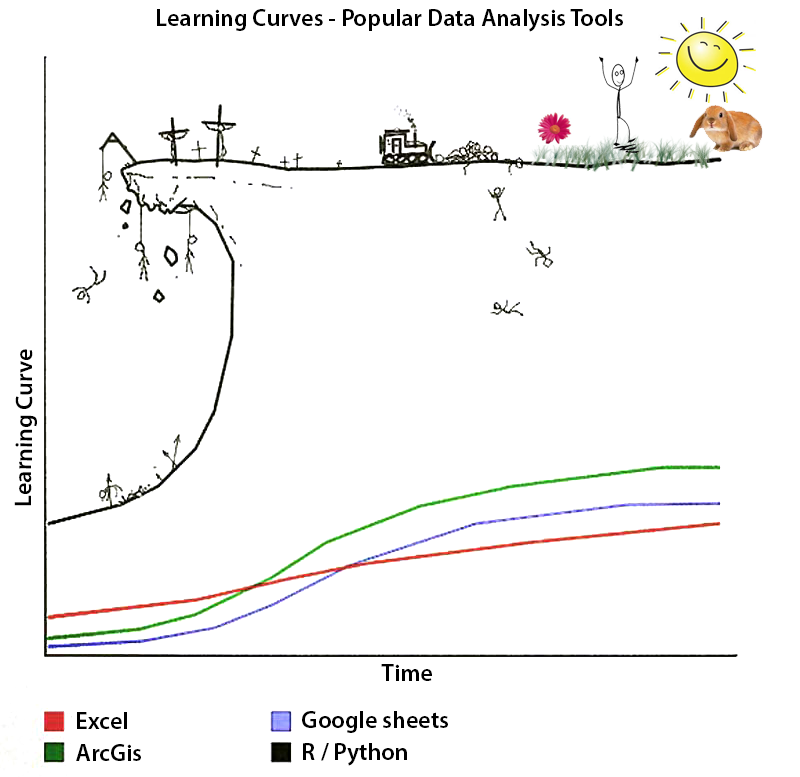
If you are already familiar with Python programming, feel free to skip to the next section. If this is your first time programming, don’t worry if some concepts seem unfamiliar or challenging. Programming can have a steep learning curve, and you’ll be surprised at how much you can accomplish in a short time.
Even if you are already familiar with Python basics, reviewing the fundamentals can be a valuable exercise, especially if your Python training was largely hands-on. I improved my understanding of programming with Python while writing this introduction. Revisiting these core concepts may be beneficial for you as well.
1.1 What is Python?
Python is a high-level, general-purpose programming language designed by Guido van Rossum in the late 1980s. It acts as a translator, abstracting away the details of computers and enabling us to communicate with them using a language that’s easier for humans to understand.
Python emphasizes readability, making it straightforward to write and understand code. It supports various programming paradigms, including procedural, where we provide a sequence of instructions; object-oriented, where we create objects with data and perform actions on them; and functional programming, where code is organized around functions.
With a vast ecosystem of libraries and frameworks, Python is widely used across diverse applications, from web development and data analysis to artificial intelligence and scientific computing. Over the years, Python has transitioned from a specialized scientific computing language to a key player in data science, machine learning, and software development, thanks to its extensive open-source libraries and its adaptability to construct sophisticated data applications.
1.2 Jupyter Notebooks
We will interact with Python code through Jupyter Notebooks on VSCode. Jupyter Notebooks, as well as the popular Jupyter Lab, are all part of the Jupyter Project, which revolves around the provision of tools and standards for interactive computing across different programming languages (Julia, Python, R) through computational notebooks.
Computational notebook, like Jupyter Notebooks, merge code, plain language explanations, data, and visualizations into a shareable document. Therefore, a notebook provides a fast and interactive platform for writing code, exploring data, creating visualizations, and sharing ideas. In other words, we can consolidate the entire data workflow behind our analysis into a single file (a notebook). This computational approach is based on the belief that hands-on interaction with code is the most effective way to learn and program.
At the end of the day, notebooks capture interactive session inputs and outputs along with explanatory text, providing a comprehensive computational record. The notebook file, saved with the .ipynb extension for Jupyter ones, is internally a set of JSON files, allowing for version control and easy sharing. Additionally, notebooks are exportable to various static formats.
Therefore, notebooks replace traditional console-based interactive computing by introducing a web-based application that captures the entire computation process, from code development and documentation to execution and result communication. The Jupyter Notebook integrates two elements:
A web application (although I recommend VSCode rather than the browser-based extension): This browser-based editing program enables interactive authoring of computational notebooks, offering a swift environment for code prototyping, data exploration, visualization, and idea sharing.
Computational Notebook documents: These shareable documents combine computer code, plain language explanations, data, visualizations, and interactive controls.
The Jupyter notebook interacts with kernels, which are implementations of the Jupyter interactive computing protocol specific to different programming languages. In plain words, kernels are the separate process that interprets and executes our code in a given programming language.
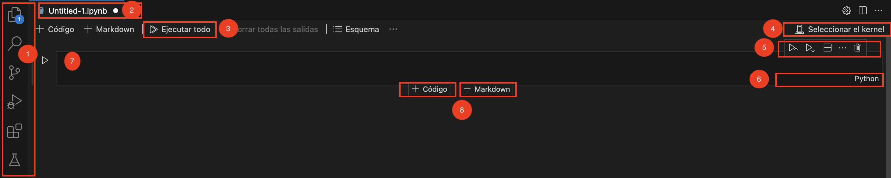
From Jupyter on VSCode we can open a new Jupyter Notebook on File → New File → Jupyter Notebook. When we open a new notebook, we will find the following elements:
Notebooks on VSCode
Toolbar of VSCode.
Name of our new notebook: notice that when a white point appears, it is because there are unsaved changes. Notice that notebooks have the .ipynb extension.
Run all: will run all cells of the notebook sequentially.
Kernel: allows us to specify the kernel where we want to run our notebook.
Notebook toolbar: allows to run and edit cells.
Indicator of type of cell (Python or markdown)
Cell
Add new cells
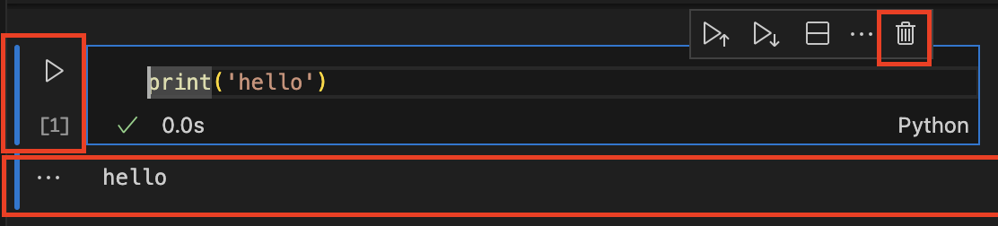
The notebook is composed of a series of cells, each acting as a multiline text input field. These cells can be executed by pressing Shift-Enter, clicking the “Play” button in the toolbar, or selecting “Cell” and then “Run” from the menu bar. The behavior of a cell during execution depends on its type, with three main types: code cells, markdown cells, and raw cells. By default, every cell starts as a code cell, but its type can be changed using a drop-down menu in the toolbar. This menu becomes active when you click on the cell type indicator in the bottom-left corner of the cell (e.g., where it says “Python” in the image below).
Notebooks on VSCode
Main types of cells:
Code cells: allow you to edit and write new code with syntax highlighting and tab completion. The programming language used depends on the kernel, with the default kernel (IPython) executing Python code.
When a code cell is executed, its computation outputs are displayed in the notebook as the cell’s output. This output can include text, matplotlib figures, HTML tables (such as those used in pandas for data analysis), and more.
Markdown cells: let you document the computational process in a literate manner by combining descriptive text with code. In IPython, this is done using the Markdown language, which provides a simple way to emphasize text, create lists, and structure documents with headings.
Headings created with hash signs become clickable links in the notebook, offering navigational aids and structural hints when exporting to formats like PDFs. When a Markdown cell is executed, the Markdown code is converted into formatted rich text, and you can also include arbitrary HTML for further customization.
Raw cells: allow you to write output directly without it being evaluated by the kernel when the notebook is run. They are useful for including preformatted text or code that should not be processed or executed.
Workflow:
A workflow in a Jupyter Notebook runs sequentially. As in a script, there is a line hierarchy within cells and a sequential hierarchy between cells. However, notebooks offer the advantage of allowing edits of cells separately multiple times until achieving the desired outcome, rather than rerunning separate scripts.
When working on a computational problem, you can organize related ideas into cells and progress incrementally, moving forward once previous parts function correctly, which is very useful when running codes that have snippets that take long. If, at any point, we want to interrupt running a cell, we can achieve that by pressing the interrupt cell. Also, we can restart the kernel to shut down the computational process.
When we run a cell, the notebook sends that process to the kernel and prints directly the execution output. The execution order appears in square brackets to the left of the printed output. Notice that when we run a notebook, all cells run in the same kernel. This means that whatever we run in a given cell will remain active unless we restart the notebook.
Also, whenever we shut down a notebook (either by restarting the kernel or just saving and closing the notebook), all of our processes and outputs that have not been saved to disk will be erased.
My tip
While notebooks are highly useful for writing and explaining work processes, particularly to other people, they may not be as practical for large research projects. Instead, I often work concurrently on a script that I run in a notebook, executing it step by step until all lines of code run smoothly. Once I have finished the code, I only save the script and run it in the terminal.
1.3 Bascis of Python syntax
Python syntax is determined by the fact that Python is:
Python is an interpreted language. By this, we mean that the Python interpreter will run a program by executing and evaluating one line at a time and sequentially. In other words, the source code is executed by the interpreter line-by-line without the need for compilation into machine code beforehand.
Python is an object-oriented programming language. Everything we define in our code exists within the interpreter as a Python object, meaning it will have its associated attributes and methods.
Attributes are values associated with an object. The class of an object defines which attributes it will have. Typically, we call objects with the syntax object.attribute_name.
Methods are functions associated with objects and can access the objects’ attributes. Typically, we use methods with the syntax object.method_name().
For instance:
x =5.2print('What part of X is real?', x.real) # This is an attribute of the variable x print('Is x an integer?', x.is_integer()) # this is a methodprint('What type of variable is x?',type(x)) # this is a function
What part of X is real? 5.2
Is x an integer? False
What type of variable is x? <class 'float'>
1.3.1 Creating variables
Important
Nothing prevents Python from rewritting variables. So if we first do x=5 and then x=6 we will automatically rewrite the variable x to 6.
Variables allow assigning names to objects stored in memory for use in our program. This call-by-object reference system means that once we assign a name to an object, we can access the object using that reference name. For example, in the code snippet above, the variable 'x' is referencing the memory object storing 5.2. We can create a new variable x2 that contains the same elements as x:
x2 = xx2
5.2
Both variables are the same because they are both referring to the same memory object. However, because numbers are immutable objects, changes to one will not affect the other.
x2 = x2 +5print("This is 'x2' variable after we sum 5 to it:", x2)print("This is our originary 'x', which hasn't changed", x)
This is 'x2' variable after we sum 5 to it: 10.2
This is our originary 'x', which hasn't changed 5.2
Strings and tuples (more on this later) are also immutable objects, but there are also mutable objects like lists. In the case of mutable objects, if we create two variables referencing the same, changing one will affect the other because both variables refer to the same memory object that has been modified.
y = ['abc','def']y2 = yy2.append('ghi')print("This is 'y2' variable after we add a new string:", y2)print("This is our orignary 'y', but...", y)
This is 'y2' variable after we add a new string: ['abc', 'def', 'ghi']
This is our orignary 'y', but... ['abc', 'def', 'ghi']
print(y)
['abc', 'def', 'ghi']
We can also assign variable names to different objects in the same code line, separating them through commas.
Just as in writing regular text, coding also involves an idiosyncratic coding style that often results in differences between two individuals’ codes, even if they are accomplishing the same task or using the same functions. This divergence is especially noticeable in variable naming. However, whether we are more of a concise or descriptive type, there are some rules and good practices for everyone:
Warning
Python is case sensitive, meaning that variables with different capitalization are considered distinct (i.e., Abc, abc, and ABC are all different)
Names can only contain upper and lower case letters, underscores (_),and numbers.
Names can never start with a digit number, only letters or or underscores.
They cannot be keywords (Python language reserved words) (help(keywords) will show which words are).
We typically use only lowercase letters for variables and reserve uppercase letters for parameters or constants.
Names should be self-explaining and balance out brevity and explicability. Typically, we reserve names for variables, verbs for attributes, and adjectives for booleans (true/false variables).
We can use names in any language, but in general, English is preferred so that anyone can follow the code.
Avoid using built-in function names because that will overwrite the function (i.e., if we write type we will no longer be able to use type to access the `type’ of variables).
1.3.3 Data types
Unlike some other programming languages, Python dynamically infers the type of a variable based on the assigned value. We can access the type of variables using the type() function.
Primitive data types are strings, integers, floats, booleans, and None. While I am hard-coding some examples for booleans, it’s more common for them to be generated as the outcome of assessing a condition within a function (i.e., Am I Alba? True). In fact, booleans are typically obtained by comparisons and can be manipulated with logical operations (and, not, or)
Besides the primitive datatypes, there are also containers datatypes. Containers are a collection of objects with a particular given structure. They can be tuples, lists, or dictionaries.
Tuples:
Fixed sequence of immutable Python objects. They are defined as a sequence of elements, separated by a comma between brackets (()), and can mix primitive data types.
We can access its elements using indexing, which we call as name_of_tuple[i], where i indicates the position of the element we want. From left to right, we start counting from 0 on the first element. From right to left, we start counting on (-1) as the last.
Note
Notice that for Python, the = is not the mathematical equality sign. It simply establishes an assignment saying the left-hand side is the right-hand side. When we want to make comparisons to check equality, we use ==.
TypeError: 'tuple' object does not support item assignment
While tuples are immutable (don’t support item assignment), we can operate with them in different ways. We can concatenate them using the + sign, we can repeat them an n number of times using *n*, and we can unpack them.
print(this_is_tuple + this_is_tuple_str + this_is_tuple_mix) # concatenatingprint(this_is_tuple_mix*3) # repeating unpack1, unpack2, unpack3 = this_is_tuple_str # unpack print(unpack1)#If we use `*_` in the unpack, we will discard some elements*_,only_third_e, a = this_is_tuple # unpack print(only_third_e)
Modifiable sequence of mutable Python objects (i.e., a tuple that we can change). They are also defined as a comma separated sequence of elements, but differently from tuples, with square brackets ([]).
print(this_is_list[2]) # 3rd elementprint(this_is_list[0:2]) # starts at 0, ends at 2-1 (i.e., 1 which is the second element)
['a', True]
['a', 4]
We can extend them, using append() and, also, we can modify them by inserting elements in specfic positions using insert(positions,what we want to insert).
this_is_list.insert(2,'Hola')print(this_is_list)
['a', 4, 'Hola', ['a', True]]
this_is_list.append(['a','b','c'])print(this_is_list)this_is_list.append('hello')print(this_is_list)# let's inset hola as the second elementthis_is_list.insert(2,'Hola')print(this_is_list)
Unordered collection of items. Items consist on pairs of Python objects named keys and values. Each key is associated with a unique value, like in a dictionary entry, which allows accessing, retrieving and modifying its values. Dictionaries are typically created using curly braces as {key1:value1,key2:value2}.
weekday_activities = {"Monday": ["Go to work", "Attend meetings", "Exercise", "Cook dinner"],"Tuesday": ["Work on projects", "Run errands", "Visit the gym"],"Wednesday": ["Work remotely", "Attend class", "Grocery shopping"],"Thursday": ["Client meetings", "Volunteer", "Cook dinner"],"Friday": ["Finish work tasks", "Meet friends for dinner", "Movie night"],}
weekday_activities['Monday']
['Go to work', 'Attend meetings', 'Exercise', 'Cook dinner']
To access one of the elements, we can look for the corresponding key.
We can also obtain all keys and values, through methods keys(), values(), items(). The results of these methods, although they migh seems like lists, cannot be subscripted.
To add extra elements to an existing entry, we can use append. However, to be able to have this funcionality we should always write the values of the entries as list (i.e., in square brackets [])
Using items() we iterate through each entry in the dictionary. To do this, for each entry, we unpack the two elements that appear in the tuple generated by .items()
for keys, values in weekday_activities.items():print('My schefule for', keys, 'is', values)
My schefule for Wednesday is ['Work remotely', 'Attend class', 'Grocery shopping']
My schefule for Thursday is ['Client meetings', 'Volunteer', 'Cook dinner']
My schefule for Friday is ['Cinema', 'Dinner out']
My schefule for Saturday is Fondue night
My schefule for Sunday is Hike
Also, if we have a collecion of keys and values, we can write them as a dictionary using .zip(k,v). This will automatically assign the keys to the values in an ordered manner (i.e., first element of the key list cooresponds to first element of the value list).
Sometimes, our code repeats the same few lines multiple times, or we are sharing the same lines in different scripts. Functions in Python allow us to encapsulate a set of instructions and reuse them throughout our code. This helps us avoid repeating the same code multiple times and makes our code more organized and easier to maintain while the complexity of the function is abstracted away.
In essence, functions contain three elements: the arguments, the commands we execute on them (i.e., the body of the function), and the return values. They have the following structure:
def function_name(arg1, arg2):# do something with argument 1 and argument 2 to get the result r3return r3
It is also possible to avoid returning anything by specifying return None or nothing at all or even using print() expressions.
Although a function can have multiple returns, it cannot have more than one return line (unless they are part of some conditions) because the function stops evaluating the code after it reaches the first return.
Notice if we call as an argument a variable that has been defined outside the function, it will automatically take that value (i.e., it’s global to the function). If the variable is also defined inside, it will be local within the function.
global_var =10def example_function(global_var):# Access and modify the global variableprint("Input you gave me", global_var) global_var = global_var +5# Modify the global variableprint("Inside the function - modified global_var:", global_var) # Call the functionexample_function(global_var)print("Outside the function - global_var:", global_var) # Call the functionexample_function(7)print("Outside the function - global_var:", global_var)
Input you gave me 10
Inside the function - modified global_var: 15
Outside the function - global_var: 10
Input you gave me 7
Inside the function - modified global_var: 12
Outside the function - global_var: 10
1.3.5 Control flow: branching and looping.
Every script and computer program generally consists of instructions that are executed sequentially from top to bottom. This sequence is referred to as the program’s flow. It is possible to alter this sequential flow to include branching or repeating certain instructions. The statements that enable these modifications are collectively known as flow control.
1.3.5.1 Branching: if, elif, else
Branching refers to the capacity to make decisions and execute distinct sets of statements depending on whether one or more conditions are met. In Python, branching departs from the if statement.
if condition:
    do line1
    do line2
Whenever the condition is found to be true, the code will perform line1 and line2. The way Python understands line1 and line2 are associated with the if statement is because of identation (i.e., white space to the left of the beginning of a line). The 4 spaces from the left to where do line1 is written constitute the Python ident. We can use the tab key to get the ident and shift+tab to remove one ident. Idents are cumulative, so if we had two blocks, the lines within the second would have to have two idents.
For instance, the line below would perform line1 only if the condition is true, and after it would perform line2 for all.
if condition: do line1do line2
month ='January'if (month=='January') or (month=='February'):print('Hey, you are in the idented block')print('The entire month of', month, ' is considered to be in the winter')
Hey, you are in the idented block
The entire month of January  is considered to be in the winter
month ='June'if (month=='January') or (month=='February'):print('Hey, you are in the idented block')print('The entire month of', month, ' is considered to be in the winter')
But what if we still want our branch to do something when the first condition is not met? We can achieve this by specifying a new action with else:
if condition1: do line1else: do line2
Notice that, whenever condition1 is not true, the else condition will imply we perform line2.
month ='May'if (month=='January') or (month=='February'):print('Hey, you are in the idented block')print('The entire month of', month, 'is considered to be in the winter')else: print('The entire month of', month, 'is NOT considered to be in the winter')
The entire month of May is NOT considered to be in the winter
We can also be more specific and chain conditions using elif. This will start executing the first condition, if it is not true, it will try the second, and so on and so forth. Once it has found a condition for which it is True it will execute the lines under it and will stop evaluating the rest of the conditions. This means that at most one - the first encountered- True statement will be evaluated.
month ='May'if (month=='January') or (month=='February'):print('Hey, you are in the idented block 1')print('The entire month of', month, 'is considered to be in the winter')elif (month=='April') or (month=='May'): print('Hey, you are in idented block 2')print('The entire month of', month, 'is considered to be in the spring')elif (month=='July') or (month=='August'): print('Hey, you are in idented block 3')print('The entire month of', month, 'is considered to be in the summer')elif (month=='October') or (month=='November'): print('Hey, you are in idented block 4')print('The entire month of', month, 'is considered to be in the autumn')else:print('Hey, you reached the else')print('The month', month, 'is in between two different seasons')
Hey, you are in idented block 2
The entire month of May is considered to be in the spring
month ='January'if (month=='January') or (month=='February'):print('Hey, you are in the idented block 1')print('The entire month of', month, 'is considered to be in the winter')if month=='January':print('We are in the nested if')print("It's cold")elif (month=='April') or (month=='May'): print('Hey, you are in idented block 2')print('The entire month of', month, 'is considered to be in the spring')elif (month=='July') or (month=='August'): print('Hey, you are in idented block 3')print('The entire month of', month, 'is considered to be in the summer')elif (month=='October') or (month=='November'): print('Hey, you are in idented block 4')print('The entire month of', month, 'is considered to be in the autumn')else:print('Hey, you reached the else')print('The month', month, 'is in between two different seasons')
Hey, you are in the idented block 1
The entire month of January is considered to be in the winter
We are in the nested if
It's cold
If we want a statement to do nothing in Python, we use the pass keyword. This is because Python does not allow an empty block within a conditional statement. It’s akin to being at a crossroads where we have to choose between turning left or right, but instead, we decide to wait and take no action.
month ='April'if (month=='January') or (month=='February'):print('Hey, you are in the idented block 1')print('The entire month of', month, 'is considered to be in the winter')elif (month=='April') or (month=='May'): passelif (month=='July') or (month=='August'): print('Hey, you are in idented block 3')print('The entire month of', month, 'is considered to be in the summer')elif (month=='October') or (month=='November'): print('Hey, you are in idented block 4')print('The entire month of', month, 'is considered to be in the autumn')else:print('Hey, you reached the else')print('The month', month, 'is in between two different seasons')
1.3.5.2 Looping: while, for
Sometimes, we also want to repeat the same statement multiple times. This is what we mean when we refer to iteration or looping, which we achieve in python through while and for.
While loops execute a statement whenever the condition is true. We typically use this kind of loop to perform some operation or update in the variable.
Good morning, Joël!
Good morning, Alba!
Awesome! Enjoy your class
Notice that the previous loop would go on and if we hadn’t written the good_morning ='N'. That’s why typically in while loops we update the variable to make sure we stop when we reach a given amount of iterations. In the Notebook version of this section, you’ll be requested to input ‘Y/N’ in the loop so that you can see that unless you press ‘N’ it will continue runing.
Good morning, Joël!
Good morning, Alba!
Good morning, Joël!
Good morning, Alba!
Good morning, Joël!
Good morning, Alba!
Awesome! Enjoy your class
For loops are used to iterate over elements of a sequence. For instance, in the first example, I will loop over the elements in ‘Cemfi’ and return each of them as an upper case letter.
for i in"Cemfi":print(i.upper())
C
E
M
F
I
months_of_year = ["January", "February", "March", "April", "May", "June", "July", "August", "September", "October", "November", "December"]# Loop through the months and add some summer vibesfor month in months_of_year:if month =="June":print(f"Get ready to enjoy the summer break, it's {month}!")elif month =="July":print(month,"is perfect to find reasons to escape from Madrid") elif month=='August': # the \n allows to break the print in two linesprint(month, 'is when you realize that living in Madrid is like living\n6 months in winterfell and 6 months in winterHELL\n') print('The joke in spanish makes more sense and is unrelated to GoT: 6 meses de invierno y 6 meses en el infierno') else:print(f"Winter is coming")
Winter is coming
Winter is coming
Winter is coming
Winter is coming
Winter is coming
Get ready to enjoy the summer break, it's June!
July is perfect to find reasons to escape from Madrid
August is when you realize that living in Madrid is like living
6 months in winterfell and 6 months in winterHELL

The joke in spanish makes more sense and is unrelated to GoT: 6 meses de invierno y 6 meses en el infierno
Winter is coming
Winter is coming
Winter is coming
Winter is coming
The function range generates a sequence of number to loop over. It follows the syntax range(start, stop, step):
Start is optional and it starts from 0 unless otherwise specified.
Stop: is always needed. The last number will always be stop-1
Step: optional, defaults to 1.
for i inrange(10):print(i+2)
2
3
4
5
6
7
8
9
10
11
1.4
A module in Python is a program that can be imported into interactive mode or other programs for use. A Python package typically comprises multiple modules. Physically, a package is a directory containing modules and possibly subdirectories, each potentially containing further modules. Conceptually, a package links all modules together using the package name for reference.
NumPy (Numerical Python) is one of the most common packages used in Python. In fact, numerous computational packages that offer scientific capabilities utilize NumPy’s array objects as a standard interface for data exchange. That’s why, although NumPy doesn’t inherently have scientific capabilities, understanding NumPy arrays and array-based computing principles can save you time in the future.
NumPy offers many efficient methods for creating and manipulating numerical data arrays. Unlike Python lists, which can accommodate various data types within a single list, NumPy arrays require homogeneity among their elements for efficient mathematical operations. Utilizing NumPy arrays provides advantages such as faster execution and reduced memory consumption compared to Python lists. With NumPy, data storage is optimized through the specification of data types, enhancing code optimization.
import numpy as np
The array serves as a fundamental data structure within the NumPy. They represent a grid of values containing information on raw data, element location, and interpretation. Elements share a common data type, known as the array dtype.
One method of initializing NumPy arrays involves using Python lists, with nested lists employed for two- or higher-dimensional data structures.
a = np.array([1, 2, 3, 4, 5, 6])
We can access the elements through indexing.
a[0]
1
Arrays are N-Dimensional (that’s why sometimes we refer to them as NDarray). That means that NumPy arrays will encompass vector (1-Dimensions), matrices (2D) or tensors (3D and higher). We can get all the information of the array by checking its attributes.
print('Dimensions/axes:', a.ndim)print('Shape (size of array in each dimension):', a.shape)print('Size (total number of elements):', a.size)print('Data type:', a.dtype)
Dimensions/axes: 2
Shape (size of array in each dimension): (2, 6)
Size (total number of elements): 12
Data type: int64
We can initialize arrays using different commands depending on what we are aiming at.
For instance, the most straightforward case would be to pass a list to np.array() to create one:
arr1 = np.array([5,6,7])arr1
array([5, 6, 7])
However, sometimes we are more ambiguous and have no information on what our array contains. We just need to be able to initialize an array so that later on, our code, can update it. For this, we typically create arrays of the desired dimensions and fill them with zeros (np.zeros()), ones (np.ones()), with a given value (np.full()) or without initializing (np.empty()).
Tip
When working with large data, np.empty() can be faster and more efficient. Also, large arrays can take up most of your memory and, in those cases, carefully establishing the dtype() can help to manage memory more efficiently (i.e., chose 8 bits over 64 bits.)
from numpy import zeros as nanazeros
nanazeros(4)
array([0., 0., 0., 0.])
np.ones((2,2))
array([[1., 1.],
       [1., 1.]])
Here you have an example of a 3D array of ones: if has 3 rows, 2 columns and 1 of height (depth)
np.ones((3,2,1))
array([[[1.],
        [1.]],

       [[1.],
        [1.]],

       [[1.],
        [1.]]])
We can use np.full() to create an array of constant vales that we specify in the fill_value option.
np.full((2,2,) , fill_value=4)
array([[4, 4],
       [4, 4]])
When we use np.empty() we are creating an unitialized array, in the sense that it is reserving the requested space in memory and returns an array with ‘garbage’ values.
np.empty(2)
array([-1.53282543e-270, 2.96171364e-036])
With np.linspace() we create an array with values that are equally spaced between the start and endpoint. For instance, in the below code we are creating an array with 5 equally spaced values from 0 to 20.
np.linspace(0,20,num=5)
array([ 0., 5., 10., 15., 20.])
1.4.0.1 Managing array elements.
Arrays accept common operations like sorting, concatenating and finding unique elements.
For instance, using the sort() method we can sort elements within an array.
arr1 = np.array((10,2,5,3,50,0))np.sort(arr1)
array([ 0, 2, 3, 5, 10, 50])
In multidimensional arrays, we can sort the elements of a given dimension by specifying the axis (0 within columns, 1 across rows)
mat1 = np.array([[1,2,3],[8,1,5]])mat1
array([[1, 2, 3],
       [8, 1, 5]])
mat1.sort(axis=0)mat1
array([[1, 1, 3],
       [8, 2, 5]])
Using concatenate we can join the elements of two arrays along an existing axis.
count # First element appears 3 times, second 1...
array([3, 1, 2, 1, 1, 1, 1, 2])
Comparing NumPy arrays is can be done using operators as ==, !=, and the like. Comparisons will result in an array of booleans indicating if the condition is met for the cells.
From algebraic rules, we can only perform operations on an array and a scalar or with two arrays of the same shape. NumPy arrays support common operations as addition, substraction and multiplication as long as those two conditions are met.
For NumPy, operations that happen within cells are what we know as broadcasting. Broadcasting is how NumPy operates between two arrays with different numbers of dimensions but compatible shape.
Element-wise addition, substraction and multiplication can be performed with +, - and *.
arr1+arr2
array([[11, 22, 33],
       [44, 55, 66]])
arr1-arr2
array([[ -9, -18, -27],
       [-36, -45, -54]])
arr1*arr2
array([[ 10,  40,  90],
       [160, 250, 360]])
To multiply (*) or divide (/) all elements by an scalar, we just specify the scalar.
arr1*10
array([[10, 20, 30],
       [40, 50, 60]])
arr2/10
array([[1., 2., 3.],
       [4., 5., 6.]])
Matrix multiplication is achieved with matmul(). Because both of our matrices are 3-by-2, I will transpose one of them so that we can perform matrix multiplicaiton.
np.matmul(arr1,arr2.T)
array([[140, 320],
       [320, 770]])
1.5 Practice exercises
Create a 1D array with all integer elemenets from 1 to 10 (both included). No hard-coding allowed!
Show solution
array_ex = np.array(range(1,11))
From array you created in 1, create one that contains all odd elements and one with all even elements.
Show solution
odds = [o for o in array_ex if o%2==1]even = [o for o in array_ex if o%2==0]
Create a new array that replaces all elements in 1 that are odd by -1.
Create a 3-by-3 matrix filled with ‘True’ values (i.e., booleans).
Show solution
mat3 = np.full((3,3),fill_value =True,dtype=bool)#Congrats! you just created your first mask
Suppose you have array a=np.array(['a','b','c','d','e','f','g']) and b = np.array(['g','h','c','a','e','w','g']). Find all elements that are equal. Can you get the position where the elements of both arrays match?
Write a function that takes a element an array and prints elements that are divisible by a given number. Try it creating an array from 1 to 20 and printing divisibles by 3.
Show solution
def print_divisible(array,div):for i in array: if i%div ==0:print(i,'is divisible by', div)returnNonearr =np.array(range(1,21))# call the function#print_divisible(arr,3)
Consider two matrices, A and B, both of size 100x100, filled with random integer values between 1 and 10. Implement a function to perform element-wise multiplication of these matrices using nested loops. Implement the same operation using Numpy’s vectorized multiplication. Repeart again with matrices of size 1000x1000, 10000x10000, 1000000x1000000 and compare the execution time. Which one is faster?
Show solution
mat_a =np.random.randint(1, 11, size=(1000, 1000))mat_b =np.random.randint(1, 11, size=(1000, 1000))def multiply_in_loop(m1,m2):if m1.shape != m2.shape:raiseValueError("Matrices A and B must have the same shape.") m, n = m1.shape result = np.zeros((m, n))for i inrange(m):for j inrange(n): result[i, j] = m1[i, j] * m2[i, j]return resultout= multiply_in_loop(mat_a,mat_b)out_built = np.multiply(mat_a,mat_b)# to check each element is exactly the same(out_built == out).sum()